| Evaluating Receive Antennas with a Soundcard |
Some work really well, others very disappointingly. But why? Without objective measurement, it's all arm-waving and opinion. But in-situ measurement of fixed antennas has hitherto been practically impossible.
Well, we'll soon fix that.
There are three contributory subjects that need a bit of introduction before they later intersect. We'll then walk through the measurement technique, a discussion of what can be done to improve the antennas in the light of the results, highlighted by a couple of special case situations.
First Introductory Subject - directional receive antennas!
|
|
Then along came NEC-based antenna computer modelling software, with feverish beavering in many a shack, affording a rash of promising new antenna designs. Schisms between those who swore by computer modelling and those who swear at it, and between those whose antennas worked and those whose never seemed to, grew deep and wide. What has been missing has been an independent way of measuring actual real-world antennas, in order to help defuse the polarisation.
Nearly all the newly re-invented compact receive antennas derive from the terminated loop, the earliest reference to which I've found was in an appallingly mimeographed prewar training manual of my Dad's, transcribed as Fig.1. It was in the form of a circular loop with a feedpoint one side and a terminating resistor the other. It is cardioid (literally, 'heart-like') in azimuthal response, and very broadband, maintaining its directivity over many octaves. It was mentioned in the context of the far better known technique of summing a conventional loop's output (figure-8 response) with that of a co-located vertical 'sense' antenna (omni) to achieve a cardioid response.
In the terminated loop, if the termination is zero (shorted) then the loop acts as, well, a loop with its well-known figure-8 response; if the termination is opened then it acts as merely a 'halo' bent dipole, with a substantially omnidirectional response in the horizontal plane; with the termination resistor value at some point in between, the balanced 'mix' of conventional loop and dipole responses, figure-8 and omni, result in a cardioid response, just as with the loop-and-sense arrangement. Why didn't the terminated loop hit the big-time before? Because the small sized, non-resonant loop and the termination resistance make the antenna lossy, inefficient and insensitive. But such trifles have never got in the way of us hambones.
The 'Ewe' (Fig. 2, top left), perhaps the best well-known of the genre after being introduced by Floyd Koontz in 'QST' magazine, can be considered exactly half that loop, using ground as the divider and return. Fig.2, top middle is an elevated Ewe, wire replacing the ground return. The 'imbalance' of termination and feedpoint hardly affects the theoretically available cardioid pattern at all. Indeed the K9AY (Fig.2, bottom right) brings the termination and feedpoint right together, (dramatically easing direction switching etc.) but does demand a ground or plane at that point as a potentiometric separator. Again, near identical cardioid. Same with the 'Flag' and 'Pennant' (owing to Earl, K6SE), the 'Kaz' (Neil Kazaross, a prominent medium-wave DXer) and pretty much every other elevated terminated loop (ETL).
The many and various designs have next to nothing to choose between them for pattern (do I have to say 'cardioid' even once more?) but play variously to ease of installation, size, ready direction switching, and/or relatively constant impedance and/or accurate tracking of nulls over broad bandwidth. As for the last two, it is of little consequence what the antenna 'looks like' to the receiver, the 'broadband' designs hold their patterns little better than any of the other designs, and those with theoretically deeper or wider nulls tend to wash out in the real world, particularly if the terminations are not carefully trimmed. They all differ in (very) minor response detail, since none of them are infinitesimally small in wavelength. Again, although tidy minds might rebel at the seeming asymmetry of the 'Elevated Ewe', Fig.2 top centre, versus the 'Flag' (Fig.2, top right) there is in neither modelling nor measuring anything of difference worth mentioning. However, the 'Elevated Ewe' is considerably easier to erect and maintain.
|
Their one major strength is the potentially relatively deep null off the rear; the trick with these simple antennas is not to point them AT things one wants, but point them directly AWAY from things one doesn't.
A raw cardioid pattern, consisting of a very broad frontal lobe and a sharply defined narrow null off the rear, is pretty weedy unless one can point that null at something obnoxious. In the northeast US, ETLs with their nulls aimed towards 'static alley', Texas to Florida, prove useful. That as a consequence they end up sort-of pointing at Europe is handy, but unimportant; it's the suppressing the storm-noise that counts.
|
Terminated Loops only get really interesting though when combined in arrays; these can be 'in-line' (i.e. one in front of the other) or 'broadside', side-by-side. Optimum spacing for side-by-side on, say, topband tends to be too wide for eighty, with the 'nose' fracturing into lobes; optimum for eighty is inadequate for topband with barely improved directivity over a single antenna, so one of the big plusses - the broadband nature of the antenna - goes away. Additionally the space required - say 300 feet separation for topband - is starting to veer dangerously back towards Beverage-land.
In-line arrays can be made to track broadband much better, easily well enough over say the octave encompassing topband and eighty, but at the cost of some sensitivity, meaning non-miniature loops and preamplifiers are necessary.
|
|
So what has been the purpose of this minor exposition on terminated loop antennas? One of these 'U2' arrays, and a couple of conventional single terminated loops, were targets for the measurement technique described later. Mostly because I wanted to see if they worked as advertised (modelled), or whether I'd been fooling myself with them for the last few years!
Second Introductory Subject - Serendipitous Signals
One would think that here in the 21st. century, and with a technology as mature as AM broadcast, that it'd be possible for those transmitters to actually be on the right frequency.
"Of course, Virginia . . ."
The clue's been there all along; if one listens to a medium-wave AM broadcast channel at night with no one signal predominant, one just hears a low-frequency beating 'burble' of heterodyning carriers and mush of mixed modulations. The beating indicates the carriers are NOT in fact all on the same frequency.
Looking at a nominal channel frequency with a spectrum analyser shows this up quite readily; the carriers are often only within +/-10Hz of nominal, some stragglers even further out. One of my 'locals' is 27Hz low! Pathetic really. At night the channels are a real mess, with often in the dozens of carriers detectable; during the day it's a lot less chaotic with a manageable number of stable ground-wave signals, all plainly visible and with the right tools separable and identifiable.
Which brings us quickly crashing into the Third Introductory Subject - The Tools.
|
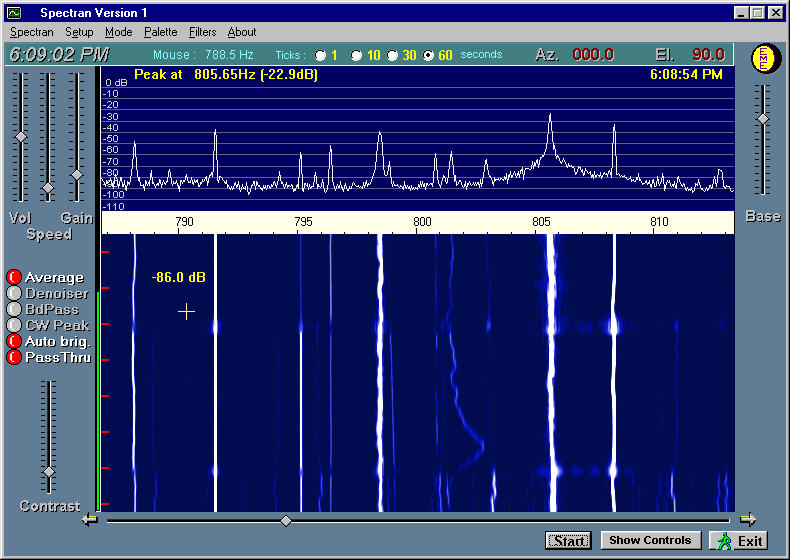
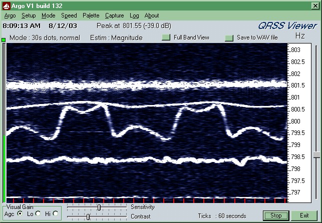
Alberto, I2PHD makes freely available 'Spectran' and a communications-optimized derivative 'Argo', and Wolf DL4YHF has his 'SpecLab' for free download, too. These are the tools that have enabled astounding progress in EME and Low Frequency (73 and 136kHz) communications. Hardly any LF 'first' has occurred in recent years not involving one of these programs.
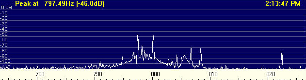
These programs run on any decent PC (all seem to work, if not perhaps to their full capability, on a 200MHz machine) and take their input from the machine's soundcard microphone or (preferably) line input. This should be fed via an isolating transformer from the fixed-low-level output from the receiver, set for either SSB or CW reception. On the displays shown here, the centre-frequency of the spectrum is at 800Hz, which just happens to be the default CW offset frequency from the radio I used. Most of these displays show +/- 13Hz from the broadcast channels' supposed nominal frequencies.
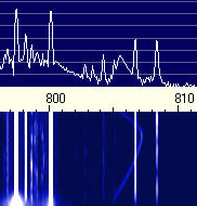
FFT analysers have it all over ordinary receivers with filters, and conventional swept spectrum analysers, since they in effect carve up the viewed spectrum with thousands of individual really narrow filters, the output of all being available for display simultaneously, typically in a rolling-time 'waterfall' display. A gee-whiz setting might call up a 256k-point (262144 'filter') at a 5.5kHz sample rate resulting in a spectral resolution of about TWO HUNDREDths of a Hertz. Typically though we'll use coarser than that in these analyses.
|
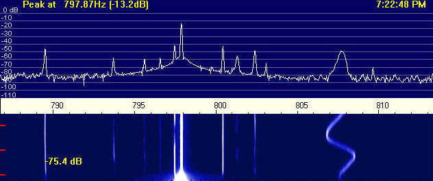
Looking at channels, in addition to the less-than-exemplary frequency management and drifting, yes, drifting carriers, one immediately starts coming across almost comical things: like the 'woodles'. There's a good one at about 808 on the plot of Fig.8.
Some carriers will show seemingly weird drifting, asymmetric wobbling or bouncing between two frequencies; this is characteristic of the frequency stabilising loops used in some broadcast transmitters. The soft saw-toothy shape is from a temperature stabilised ('ovened') crystal oscillator; it slowly drifts until the lower temperature is reached, the oven clonks on, the frequency rapidly rises, oven turns off. The good news and direct relevance for us is that it becomes really easy to repeat identify these 'offenders'; but when one starts calling them by name like pets it is a sure indicator that one doesn't get out enough.
|
So it is with ease that these FFT analysis tools can lift and separate individual broadcast carriers from a seemingly inseparable 'mush', and ease identification of many from their strength or characteristics.
Yes, but why? Why on earth would we want to do that?
Bear in mind we're not _listening_ to the radio stations, just looking at their carriers. And those carriers can be detected a long, long way off - way beyond their nominal 'service area' (to whit, KFI) - given the huge signal-to-noise ratio afforded by the analyser's narrow filters. So what we are seeing on any given broadcast channel is a whole bunch (technical term) of radiated signal sources from all sorts of places.Lots of signals. From different directions.
Choose the channel carefully, and those many stations, from those many directions, could be meaningfully dispersed around 360 degrees. If necessary, nearby channels may well contain signals coming from other useful directions to augment.
Here's the crucial part: comparing the signal level of each of those signals as received on an omnidirectional 'reference' antenna with the levels detected through a 'test' directional antenna can tell you a lot about that antenna's actual directional characteristics. The more carriers and the better their angular dispersal, the better fleshed out the picture of the antenna will become.
So, we've arrived at where the three stories collide: Real-world receive antennas of assumed (or hoped for) directional characteristics, rafts of accidental multidirectional signal sources, and tools to analyse them. Resulting in the germ of an idea to accurately measure the antennas.
The ultimate goal is a polar plot of the subject antenna's azimuth response. To do that, we need to establish the displayed frequency and azimuth for each of the signal sources, capture the reference/subject level differences, normalise them to suit the scaling, then plot them. (It's a bit of a twisty path to get there, and someone is bound to tell me that their 11-year-old daughter could whip up a quick 'Excel' script to do it all, but mine couldn't and didn't, so this was all done with pencil-and-paper. Just humour me.)
Finding Suitable Channels
The FCC in the USA maintains a wondrous webbable database of all AM broadcasting transmitters; call, location, power, distance and bearing of stations within a given radius are easily extracted. There is a similar, though independently maintained, database for European AM stations, which while not as comprehensive does have adequate information to enable one to pick likely channels and derive distance and bearings longhand. If one is prepared to don one's bureaucratic hip-waders, there's always the ITU database, of course.
A regional map of reasonable scale encompassing the likely stations, and play-time tools such as a compass, a protractor and a ruler help visualise and realise the process. It's all a bit weird in the abstract, and it's amazing how faulty guesses at bearing and distance to other towns can be!
Following is a sliced-and-diced extract from the FCC database for easily identified stations around me. Next to the frequency is an (added later by me) identifying frequency (centre is 800Hz, a ~ indicates a woodler) showing where I can find the carrier again on a 'Spectran' screen; location, power, distance, bearing and a derived (by me) approximate strength in dB below a kilowatt-kilometer. This relative level indication becomes important later. Pay attention.
1440 800   WNPV  LANSDALE        PA   2.5kW   90.97km   91.25deg  -59dB
1440 798   WMVB  MILLVILLE       NJ   1.0kW  149.46km  128.19deg  -70dB
1440 787   WTHM  RED LION        PA   1.0kW   42.86km  202.46deg  -52dB

1450 801.4 WPAM  POTTSVILLE      PA   1.0kW   50.52km   18.91deg  -55dB
1450 799   WILM  WILMINGTON      DE   1.0kW   92.57km  129.41deg  -63dB
1450 787   WOL   WASHINGTON      DC   1.0kW  159.88km  199.56deg  -71dB
1450 795   WTHU  THURMONT        MD   0.5kW  111.59km  231.14deg  -69dB
1450 800   WMAJ  STATE COLLEGE   PA   1.0kW  137.03km  296.86deg  -68dB

1460 802.5 WDDY  ALBANY          NY   5.0kW  339.63km   38.53deg  -74dB
1460 797.5 WIFI  FLORENCE        NJ   5.0kW  136.85km   97.88deg  -61dB
1460 789   WEMD  EASTON          MD   1.0kW  167.82km  170.89deg  -71dB
1460 798   WTKT  HARRISBURG      PA   5.0kW   44.35km  270.25deg  -46dB

1470 801   WKAP  ALLENTOWN       PA   5.0kW   87.06km   61.09deg  -55dB
1470 800   WJDY  SALISBURY       MD   5.0kW  217.41km  162.70deg  -68dB
1470 792   WTTR  WESTMINSTER     MD   1.0kW   93.33km  215.61deg  -63dB
1470 797   WTKO  ITHACA          NY   5.0kW  237.05km  358.28deg  -69dB

1480 800   WZRC  NEW YORK        NY   5.0kW  210.33km   71.26deg  -67dB
1480 797   WDAS  PHILADELPHIA    PA   5.0kW  104.19km  105.92deg  -58dB
1480 791   WEEO  SHIPPENSBURG    PA  0.46kW   99.66km  258.39deg  -67dB

1490 800   WAZL  HAZLETON        PA   1.0kW   83.41km   25.05deg  -61dB
1490 798   WBCB  LEVITTOWN       PA   1.0kW  132.23km   93.95deg  -68dB
1490 807   WUSS  PLEASANTVILLE   NJ   0.4kW  187.17km  120.56deg  -77dB
1490 797   WLPA  LANCASTER       PA   0.6kW   23.12km  164.65deg  -46dB
1490 806~  WARK  HAGERSTOWN      MD   1.0kW  133.01km  238.38deg  -68dB
1490 822   WNTJ  JOHNSTOWN       PA   1.0kW  212.84km  272.68deg  -74dB

1550 808   WITK  PITTSTON        PA  10.0kW  130.83km   22.62deg  -58dB
1550 800   WJRZ  TOMS RIVER      NJ   1.0kW  189.02km   99.77deg  -73dB
1550 803   WXHL  ELKTON          MD   1.0kW   89.50km  145.54deg  -62dB

1560 800   WQEW  NEW YORK        NY  50.0kW  214.94km   75.57deg  -58dB

1570 799   WISP  DOYLESTOWN      PA   5.0kW  104.32km   85.63deg  -58dB
1570 800.5 WNST  TOWSON          MD   5.0kW   94.85km  188.75deg  -56dB
1570 797   WPGM  DANVILLE        PA   2.5kW   83.08km  346.05deg  -57dB

1580 806   WGYM  HAMMONTON       NJ   1.0kW  153.04km  116.97deg  -70dB
1580 774.4 WVZN  COLUMBIA        PA   0.5kW   28.27km  194.29deg  -49dB
1580 794   WPGC  MORNINGSIDE     MD  50.0kW  160.83km  195.88deg  -54dB
1580 804   WRDD  EBENSBURG       PA   1.0kW  198.73km  278.19deg  -74dB

1590 801~  WPSN  HONESDALE       PA   2.5kW  172.39km   33.16deg  -68dB
1590 802   WPWA  CHESTER         PA   2.5kW   90.03km  117.97deg  -59dB
1590 807   WCBG  CHAMBERSBURG    PA   5.0kW  115.42km  250.30deg  -59dB

1600 791   WHOL  ALLENTOWN       PA   0.5kW   85.38km   64.14deg  -65dB
1600 798.5 WWRL  NEW YORK        NY  25.0kW  205.93km   72.47deg  -60dB
1600 809   WIBF  DOVER           DE   5.0kW  140.78km  149.26deg  -62dB
1600 797   WPDC  ELIZABETHTOWN   PA   0.5kW   20.36km  240.63deg  -45dB
Channels at the high end of the band are favourite for a couple of reasons; firstly they are closer to topband, and so little if any translation needs to occur, indeed the results often can be used directly, and secondly the higher channels tend to have lots of lower power stations on them (as opposed to just one or two behemoths), which makes for a broader spread of likely suspects on useful bearings.
Generally, looking at the database, a small number of adjacent or close channels will have a reasonable spread of the compass covered.
Identifying the stations' carriers
|
"OK, So how do I tell all those carriers apart?"
A bit of sleuthing and as a last resort, hard work. The good news is that once one has identified them the first time, it is easy subsequently. Take a 'Spectran' trace of each channel using an omni antenna, spreading the traces sufficiently to separate them yet retaining enough to use on the screen. A 160/80 vertical, or a 'bit of wire', will suffice as this reference antenna; asymmetries from 'L' top loading or whatever are very minor and at least initially can be ignored, with the assumption of 'omni'.
Some quick hints:
I always try to pick a couple of channels that have 'locals' on - these offer obvious, big, unmistakeable baseline display traces. There's PLENTY of dynamic range in the FFT displays to cope, even to get high-confidence measurements of signals even 30-40dB below the local.
This is where the channel list becomes vital. Most, meaning a half to two-thirds of prominent likely-suspect signals on an omni can be identified by loudness pecking order alone, referring to the listed kilowatt-kilometer figure. At first, I didn't believe it could be that easy! A lot can be confidently nailed down this way. True, there can be spoilers, such as close and/or powerful stations that are directional to elsewhere, but generally big remains big.
"OK. So how about the rest?"
Some traces are just a wee bit too flakey to trust, so that lets them off the hook. Disregard any in which one lacks confidence. Playing with a variety of antennas, one can often suppress a predominant signal enough to hear, yes hear, an ID from the next station down, Sometimes one can go three deep doing this. As for the others, beyond this 'armchair' sleuthing, the 'hard work' bit comes in if insufficient are yet identified. A small receiving loop is perfect for this - I've used both a 2m square tuned loop, and a 12" diameter tuned loop to good effect for this: get an FFT of a channel going and _ s l o w l y _ turn the loop until signals drop out, as they will, one or a couple at a time; note the bearings, figure out from the map or listing from where they're coming. Alternatively, having calibrated the loop bearing against one of those known big local stations, set the loop to null a particular bearing (station) of interest, and see which carrier dropped out - probably an easier technique if the 'puter isn't visible from the loop. Typically though, one will only resort to this to get high confidence in traces from stations at 'important' or hitherto missing bearings. Other mis-identifies will become apparent during plotting, and it's 'back to the drawing board' (literally) for them. A bit later on, when one has confidence in a particular receive antenna, say having already plotted it, one can use ITS known directionality to give one clues, and save waving a loop around.
Comparing the reference antenna to the subject(s)
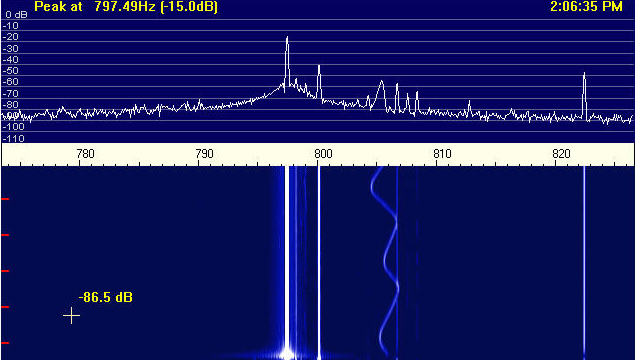
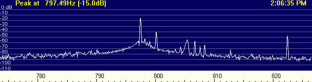
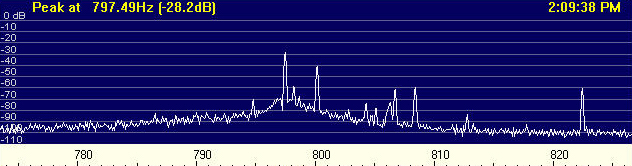
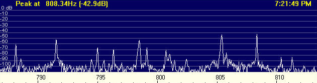
Run a 'Spectran' plot containing a chunk of the omni and each of the subject antennas, each taking say 1/3 of the waterfall screen, or about two minutes of each. Bear in mind at the narrow bandwidths of the FFT 'bins', the traces will take about a minute to settle after a change. A couple of minutes of trace is needed to permit sliding the cursor up-and-down to find a maximum; since everything is drifting (the broadcasters especially) the carriers continually cross between the exceedingly narrow FFT 'bins' (filters), and so one needs to capture them at a point when they are solidly within a single one. (This effect predominates over propagational effects by far.) 'Woodlers' are best caught as they 'turn the corner'. Here in Figs. 11,12 and 13 are screen-shots of 1490kHz from home using top, omni; middle, a single 'U' (actually the forwardmost loop of the array) and bottom, the 'U2' array. I had previously attenuated the omni's level to match that of the single 'U' for a known signal in its broad front lobe.
|
An example of how one can get fooled by otherwise seemingly big, loud, fine, upstanding traces is highlighted by Fig.14 (right). Look closely at the waterfall for the 808.5 trace, and in the spectrographs above - the initial clue was that magically the signal seemed to have got louder on the'U' than on the omni, then quieter again on the 'U2'. Odd. The waterfall shows it winking in and out; an indication that there are two - possibly more - signals within the same measurement 'bin' beating with each other. One could either ignore this trace altogether (wise) or if one were truly desperate for data points, crank up the resolution of the FFT to prise the little buggers apart, and then measure them.
Making channel 'crib sheets'
Having 'captured' a display full of squiggly lines from the reference omni and the subject antenna(s) it is time for the laborious creation of a channel crib-sheet: Having a couple of minutes captured allows one to find a good solid maximum value for each trace, sliding the cursor up and down and across each line. One wants to catch each signal at its best, and that means in some cases finding where a 'drifty' signal lands itself solidly in one of the FFT 'bins', rather than straddling a couple, or smeared across many.
I 'name' the carriers by displayed trace frequency (say, 797.2 WWSM Cleona) top to bottom, loudest to quietest, on the crib as they become identified, along with the trace values for each antenna in turn, and woodle character if there is one. That way I can find them again if I need to. Take captures from another or other channels, if necessary, and crib them, too. 1490kHz, the channel immortalised above, contains enough signals from enough directions to do a decent first-pass analysis, and nowadays I only go to other channels for more detail.
There is a strong likelyhood, unless care was taken beforehand, that there will be a disparity in scale between the general level of signals between the different antennas; take the time now to normalise them out on the cribs. Often, one'll conveniently find a station on a bearing close enough to 'on the nose' of the subject antenna(s) to calibrate against the omni.
Make the cribs as complete as possible - it'll reduce the amount of messing about with the polar plot, or trying to figure the mess out next time..
The Polar Plot.
Now, transfer the cribs to the polar plot. At this point, it is likely one'll find mistakes in station identities - their results just don't 'look right' plotted, and are usually transpositions with another station. Verify the bearings, adopt the changes, update the cribs. With tongue poking out of the corner of one's mouth, and with your favourite colour crayons, join the dots like they taught in primary school. Plotting has to be done the hard way at first, by cross-referring bearings with the stations with the data, but at that point a bit of work in preparing the polar plot with stations with channels pre-marked at the appropriate bearings can save a lot of aggro for further analyses later on. Here's one I prepared earlier . . . (Fig.15)
|
This example, is, amazingly, about as good as it gets in the real world. Don't get fooled, complacent or too excited. The antennas measured are almost ideally located, 50m from the nearest structure, 200m from anything that threatens to be close-resonant, are well-maintained and well tweaked. Unless one is *very lucky*, and the antenna, installation and environment are *ideal*, the azimuthal responses of such loops will not look much like they did in the model or book. There are three rational reponses: (1) Blame the modelling program. (2) Blame the measurements, (3) Go to the pub.
Why do some people have good luck with these antennas, and others disparage them? Sadly, really good performing ones seem rare - Why?
* Starry Eyes . . Unreal or excessive expectations
Some folk chuck a piece of wire in the air and think they've got some kind of death-ray. Even when working properly, a cardioid response is just a cardioid response. It is comparable to a two-element driven array. The only thing of directional significance is that reasonably deep null off the back - it is a one-trick pony. Frankly, nothing else has much real effect in the real world; the few dB attenuation off the sides is barely noticable in battle. It takes a properly working array of ETLs to approach the performance 'expected' from a casual glance at the azimuth response of a single loop.
* Incorrect termination
The termination resistor value MUST be trimmed in situ. It is critical. Just plonking in the 'book' or model value almost guarantees throwing away many dB of null depth, the major strength of the antenna. It is easy to do, makes so much difference, and so few do it. Cringe. I have a fairly local AM station at the high end of the band 'off-the-back' of euro-facing antennas; listening to that on a portable radio attached to the antenna, I tweak a 2kohm 10-turn pot at the termination until it nulls most.
* Insufficient feedline isolation
In addition to presenting the feedline with a suitable source impedance, the 'matching' transformer should serve to isolate the feedline from the antenna. Some do a good job, others don't. Ideally, the feedline should be dropped straight down to a decent ground connection, then a line isolator, or enough ferrite on the feedline to provide a high common-mode impedance, added before the run back to the shack, where connection is made through another transformer (to obviate ground loops). (Lest decoupling is considered fru-fru, try modelling the antenna with a random bit of wire connected to one side or the other of the feedpoint and see what happens.) Not insignificantly, any garbage picked up on the feedline as common-mode will get correspondingly turned into differential mode by the same mechanism and become inseparable from the desired signals. This is a prime method for entry of the 'squirglies'.
* Noises . . Noise coupling:
They are sensitive to nearby or crossing power-line noise. Distance is the only cure. Feedline common-mode exacerbates this, often dominates, and needs to be fixed first..
* Conductor pollution:
The biggy. These small loops are highly sensitive to 'conductor pollution', i.e. the effect of nearby wires or metal structures of any sort. These can and do warp the true cardioid response, typically degenerating that hard-won rear null. At worst, a nearby (meaning as close as 1/4 wavelength away) resonant antenna at the frequency of interest can completely destroy any hope of directionality.
As it just so happens, partly to illustrate this point, and partly because I needed yet another antenna, I installed a 'Mondo-Kaz', a single triangular loop some 40m long and 10m high in the centre with the 'live' end about 20m away from a 160m vertical, self-resonant at 1.7MHz. Here, Figs. 16,17,18 and 18 illustrate the effect of proximity. They are of nominal 1600kHz with a 'local' station (at 805.5) pretty much bang in the null behind - yes, in fact it is the signal I use to trim termination resistors - and conveniently, a signal 'on-the-nose' for reference (at 808.5). The 'Kaz' has been trimmed, to the tune of some 22dB rear rejection.
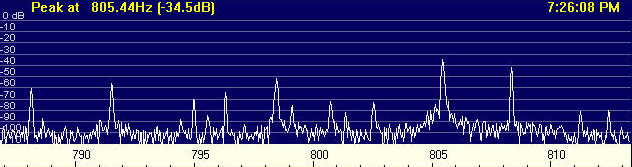
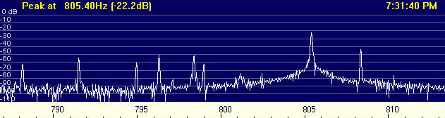
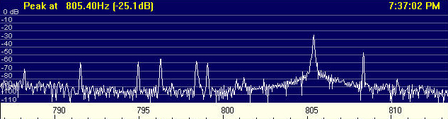
In summary
This paper has briefly outlined the development of compact terminated loop antennas, detailed a particular arrangement of a single loop, and more particularly a modestly-sized in-line phased array of loops. These two antennas were used as targets for a novel and reasonably accurate azimuth pattern evaluation technique, which relies upon multitudinous broadcast signals and modern PC-based FFT spectral analysis tools to separate and measure them. The technique allows the plotting of antennas' responses, and the ready examination of environmental effects on their behaviour.
Measuring antenna elevation responses will have to wait for the next episode of 'Mission Impossible'.