W3EEE - RSGB HF Convention talk

Evaluating Receive Antennas with a Soundcard

Introduction / Summary
Section (1) . . Receive Antennas
Section (2) . . *** Signals, and Signal Processing ***
Section (3) . . Measuring
Section (4) . . Problems and Solutions

Second Introductory Subject - Serendipitous Signals

One would think that here in the 21st. century, and with a technology as mature as AM broadcast, that it'd be possible for those transmitters to actually be on the right frequency.

"Of course, Virginia . . ."

The clue's been there all along; if one listens to a medium-wave AM broadcast channel at night with no one signal predominant, one just hears a low-frequency beating 'burble' of heterodyning carriers and mush of mixed modulations. The beating indicates the carriers are NOT in fact all on the same frequency.

Looking at a nominal channel frequency with a spectrum analyser shows this up quite readily; the carriers are often only within +/-10Hz of nominal, some stragglers even further out. One of my 'locals' is 27Hz low! Pathetic really. At night the channels are a real mess, with often in the dozens of carriers detectable; during the day it's a lot less chaotic with a manageable number of stable ground-wave signals, all plainly visible and with the right tools separable and identifiable.

Which brings us quickly crashing into the Third Introductory Subject - The Tools.

Fig.7: Spectran - a broadcast channel

Lately really good tools - in the form of PC-based Fast Fourier Transform based audio-frequency spectrum analysers - have become available, priced right. Shown in Fig.7 is a typical MF AM broadcast channel as looked at down the microscope of 'Spectran'.

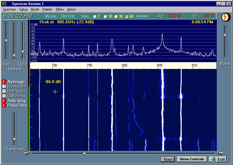
Alberto, I2PHD makes freely available 'Spectran' and a communications-optimized derivative 'Argo', and Wolf DL4YHF has his 'SpecLab' for free download, too. These are the tools that have enabled astounding progress in EME and Low Frequency (73 and 136kHz) communications. Hardly any LF 'first' has occurred in recent years not involving one of these programs.

These programs run on any decent PC (all seem to work, if not perhaps to their full capability, on a 200MHz machine) and take their input from the machine's soundcard microphone or (preferably) line input. This should be fed via an isolating transformer from the fixed-low-level output from the receiver, set for either SSB or CW reception. On the displays shown here, the centre-frequency of the spectrum is at 800Hz, which just happens to be the default CW offset frequency from the radio I used. Most of these displays show +/- 13Hz from the broadcast channels' supposed nominal frequencies.

FFT analysers have it all over ordinary receivers with filters, and conventional swept spectrum analysers, since they in effect carve up the viewed spectrum with thousands of individual really narrow filters, the output of all being available for display simultaneously, typically in a rolling-time 'waterfall' display. A gee-whiz setting might call up a 256k-point (262144 'filter') at a 5.5kHz sample rate resulting in a spectral resolution of about TWO HUNDREDths of a Hertz. Typically though we'll use coarser than that in these analyses.

Fig.8: Spectran - with a 'woodler'

On the screen, the 'Spectran' plot has a 'spectral analysis' display along the top, showing relative strengths of the various signals, whilst below it is a 'waterfall' of the analysis spread over time, 'now' at the top; the little red markers down the left-hand side indicate one minute intervals in most captures shown here . Moving the cursor around allows the easy measurement of any point on the waterfall, greatly facilitating accurate retrieval of signal level data.

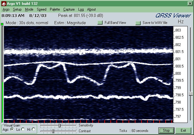
Looking at channels, in addition to the less-than-exemplary frequency management and drifting, yes, drifting carriers, one immediately starts coming across almost comical things: like the 'woodles'. There's a good one at about 808 on the plot of Fig.8.

Some carriers will show seemingly weird drifting, asymmetric wobbling or bouncing between two frequencies; this is characteristic of the frequency stabilising loops used in some broadcast transmitters. The soft saw-toothy shape is from a temperature stabilised ('ovened') crystal oscillator; it slowly drifts until the lower temperature is reached, the oven clonks on, the frequency rapidly rises, oven turns off. The good news and direct relevance for us is that it becomes really easy to repeat identify these 'offenders'; but when one starts calling them by name like pets it is a sure indicator that one doesn't get out enough.

Fig.9: 'Argo' - KFI Los Angeles

Fig.9 shows a great example. Someone on the west coast noticed that one of the Gorilla 50kW LA stations, KFI, had a *major* woodle; people literally all over the world were able to find it and take 'Argo' piccies like this one, once it was known what to look for. Additionally, at the top of the capture there is a carrier fairly typical of an AM Stereo station, with mushed phase; between it and KFI is another gentle woodler of about the same period as KFI (about 12 minutes), whilst just below KFI is a typically grotty, noisy PLL synthesiser. Oh, and there's actually a decent clean carrier near the bottom! All this type of 'character' aids repeat signal identification.

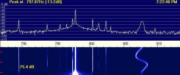
So it is with ease that these FFT analysis tools can lift and separate individual broadcast carriers from a seemingly inseparable 'mush', and ease identification of many from their strength or characteristics.

Yes, but why? Why on earth would we want to do that?

Bear in mind we're not _listening_ to the radio stations, just looking at their carriers. And those carriers can be detected a long, long way off - way beyond their nominal 'service area' (to whit, KFI) - given the huge signal-to-noise ratio afforded by the analyser's narrow filters. So what we are seeing on any given broadcast channel is a whole bunch (technical term) of radiated signal sources from all sorts of places.

Lots of signals. From different directions.

Choose the channel carefully, and those many stations, from those many directions, could be meaningfully dispersed around 360 degrees. If necessary, nearby channels may well contain signals coming from other useful directions to augment.

Here's the crucial part: comparing the signal level of each of those signals as received on an omnidirectional 'reference' antenna with the levels detected through a 'test' directional antenna can tell you a lot about that antenna's actual directional characteristics. The more carriers and the better their angular dispersal, the better fleshed out the picture of the antenna will become.

Introduction / Summary
Section (1) . . Receive Antennas
Section (2) . . *** Signals, and Signal Processing ***
Section (3) . . Measuring
Section (4) . . Problems and Solutions
Home